Parallel reductions using semidirect products
Solutions to many parallel programming problems can be reduced to a well-designed monoid[1]. As such, interesting parallel solution sometimes require non-trivial monoids. To enrich the repertoire, let us discuss semidirect product; a particularity elegant construction of useful monoids.
| [1] | Here, we mainly discuss monoid and monoid actions. However, since one can always turn a semigroup into a monoid by adjoining the identity, the following discussion also applies to semigroups which is more useful than monoid in dynamic languages like Julia. |
💡 Note
The code examples here focus on simplicity rather than the performance and actually executing them in parallel. However, it is straightforward to use exactly the same pattern and derive efficient implementations in Julia. See A quick introduction to data parallelism in Julia and Efficient and safe approaches to mutation in data parallelism for the main ingredients required.
Maximum depth of parentheses
As a motivating example, let us compute the maximum depth of parentheses in a string. Each position of a string has an integer depth which is one more larger (smaller) than the depth of the previous position if the current character is the open parenthesis ( (close parenthesis )). Otherwise the depth is equal to the depth of the previous position. The initial depth is 0. We are interested in the maximum depth of a given string:
string    (  (  (  )  )  (  )  )
depth     1  2  3  2  1  2  1  0
                ↑
                maximum depth
The following code is a Julia program that calculates the maximum depth. It computes the depth of every position using the cumulative sum function cumsum and then take the maximum of it:
parentheses = collect("(((())((()))) ((())))")
increments = ifelse.(parentheses .== '(', +1, ifelse.(parentheses .== ')', -1, 0))
depths = cumsum(increments)
maximum(depths)
5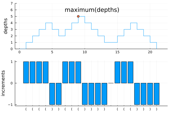
Both cumsum (prefix sum) and maximum (reduce) can be computed in parallel. However, it is possible to fuse these operations and compute the maximum depth in one sweep (which is essential for performance). To solve this problem with single-path reduction, we need to find a small set of states "just enough" for combining sub-solutions obtained by solving each chunk of the input. An important observation here is that the "humps" in the depths plot can be easily shifted up and down when combining into the result from preceding (left) string of parentheses. This motivates us to track the maximum and the final (relative) depth of a chunk of the input string. Splitting the above solution into three chunks, we get the following three sub-solutions:
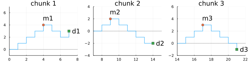
Consider chunk 1 and 2. Combining the final depths (d1 and d2) is as easy as summing these two depths. To combine the maximum in each chunk, we need to shift the right maximum m2 by the final depth of the left chunk d1 so that both maximum "candidates" m1 and m2 are compared with respect to the same reference point (i.e., the beginning of the left chunk). Thus, we get the following function for combining the solutions (d1, m1) and (d2, m2) from two consecutive chunks:
function ⊗((d1, m1), (d2, m2))
    d = d1 + d2           # total change in depth

    m2′ = d1 + m2         # shifting the maximum of the right chunk before comparison
    m = max(m1, m2′)      # find the maximum

    return (d, m)
end
Given the sub-solutions above
(d1, m1) = (3, 4)
(d2, m2) = (-2, 2)
(d3, m3) = (-1, 3)
we can compute the final result
(d1, m1) ⊗ (d2, m2) ⊗ (d3, m3)(0, 5)where the second element of the tuple is the maximum depth. As we will see in the next section, ⊗ is associative. Thus, we can use it as the input to reduce. Observing singleton chunk [x] (where x is -1, 0, or 1) has the trivial solution (x, x) (i.e., the last element of [x] is x and the maximum element of [x] is x), we get the single-sweep reduction to calculate the maximum depth of the parentheses:
mapreduce(x -> (x, x), ⊗, increments)(0, 5)Recall that mapreduce can also be computed using the left-fold mapfoldl. By manually inlining the definitions of mapfoldl(x -> (x, x), ⊗, increments), we also obtain the following sequential algorithm:
function maxdepth_seq1(increments)
    d1 = m1 = 0
    for x in increments
        d2 = m2 = x

        # Inlining `⊗`:
        d = d1 + d2
        m2′ = d1 + m2
        m = max(m1, m2′)

        d1 = d
        m1 = m
    end
    return m1
end
Since d1 + d2 and d1 + m2 are equivalent when d2 = m2 = x, we can do "manual Common Subexpression Elimination" to get:
function maxdepth_seq2(increments)
    d1 = m1 = 0
    for x in increments
        d1 = d1 + x
        m1 = max(m1, d1)
    end
    return m1
end
Note that this is the straightforward sequential solution to the original problem. Compilers such as Julia+LLVM may be able to do this "derivation" as a part of optimization in may programs. It is also possible to implement this with sufficiently rich "monoid combinator" frameworks such as Transducers.jl (using next and combine specializations).
Semidirect products (restricted version)
The structure in ⊗ of the previous section is actually very generic and applicable to many other reductions. If we replace + with *′ and max with +′, we obtain the following higher-order function (combinator) sdpl. Let us also define a similar "flipped" version sdpr.
sdpl(*′, +′) = ((a₁, b₁), (a₂, b₂)) -> (a₁ *′ a₂, b₁ +′ (a₁ *′ b₂))
sdpr(*′, +′) = ((a₁, b₁), (a₂, b₂)) -> (a₁ *′ a₂, (b₁ *′ a₂) +′ b₂)
A binary function (x, y) -> sdpl(*′, +′)(x, y) is associative (i.e., semigroup) if *′ and +′ are both associative and *′ is left-distributive over +′; i.e.,
Similarly, sdpr(*′, +′) is associative if *′ and +′ are both associative and *′ is right-distributives over +′. See, e.g., Kogge and Stone (1973), Blelloch (1990), Gorlatch and Lengauer (1997), Chauhan et al. (2016), and Kmett (2018) for the discussion and applications on this algebraic fact (or its generalized form; see below). The monoid combinator sdpl of this form in particular is described in Gorlatch and Lengauer (1997), including the proofs we skipped here. They described it as scan-reduce composition and scan-scan composition theorems. As we saw in the previous section, mapreduce(x -> (x,
x), sdpl(+, max), increments) computes maximum(cumsum(increments)) efficiently by composing (fusing) the scan (cumsum) and reduce (maximum).
Borrowing the terminology from group theory (see Semidirect product - Wikipedia), and also following Chauhan et al. (2016)'s nomenclature, let us call sdpl and sdpr the semidirect products although the definition above is not of its fully generalized form.
Other than the usual multiplication-addition pair (*, +) and addition-max pair (+, max) as discussed in the previous section, there are various pairs of monoids satisfying left- and/or right-distributivity property (see, Distributive property - Wikipedia). For example, following functions can be used with sdpl and sdpr (on appropriate domain types):
*′ | +′ | Example applications |
|---|---|---|
* | + | linear recurrence (see below) |
+ | max | maximum depth of parentheses (see above) |
+ | min | |
min | max | |
max | min | |
∩ | ∪ | unique (see below); GEN/KILL-sets |
∪ | ∩ |
The unique example (below) and GEN-/KILL-sets example in Chauhan et al. (2016) can be considered an instance of sdpl(∩, ∪) with the first monoid ∩ virtually operating on the complement sets.
Linear recurrence
Semidirect product sdpr(*′, +′) is a generalized from of linear recurrence equation:
given sequences and . Let us use the initial condition for simplicity (as specifying is equivalent to specifying ). Indeed, (1, 0) is the identity element for the method sdpr(*, +)(_::Number, _::Number). To see sdpr(*, +) computes , let us manually expand foldl(sdpr(*, +), zip(as, bs); init =
(1, 0)), as we did for maxdepth_seq1 (or, alternatively, see Blelloch (1990)):
function linear_recurrence_seq1(as, bs)
    a₁ = 1
    b₁ = 0
    for (a₂, b₂) in zip(as, bs)
        # Inlining `sdpr(*, +)`:
        a₁ = a₁ * a₂
        b₁ = b₁ * a₂ + b₂
    end
    return (a₁, b₁)
end
By eliminating a₁ and renaming b₁ to x, we have
function linear_recurrence_seq2(as, bs)
    x = 0
    for (a, b) in zip(as, bs)
        x = x * a + b
    end
    return x
end
which computes the linear recurrence equation (linrec). (Note: the first component a₁ * a₂ is still required for associativity of sdpr(*, +). It keeps track of the multiplier for propagating the effect of to .)
The above code also work when the elements in as and bs are matrices. In particular, x and b can be "row vectors." Even though Julia uses 1×n matrices for row vectors, this observation indicates that as and bs can live in different spaces. Indeed, we will see that it is useful to "disassociate" the functions for a₁ *′ a₂ and b₁ *′ a₂.
Semidirect products and distributive monoid actions
The combinators sdpl and sdpr can be generalized to the case where as and bs are of different types. We can simply extend these combinators to take three functions[2] :
sdpl(*′, ⊳, +′) = ((a₁, b₁), (a₂, b₂)) -> (a₁ *′ a₂, b₁ +′ (a₁ ⊳ b₂))
sdpr(*′, ⊲, +′) = ((a₁, b₁), (a₂, b₂)) -> (a₁ *′ a₂, (b₁ ⊲ a₂) +′ b₂)| [2] | In Julia, we acn use multiple dispatch for plumbing the calls a₁ *′ a₂ and b₁ *′ a₂ to different implementations. However, it would require defining particular type for each pair of a₁ *′ a₂ and b₁ *′ a₂. Thus, it is more convenient to define these ternary combinators.
|
(x, y) -> sdpl(*′, ⊳, +′)(x, y) is a monoid if *′ and +′ are monoids, the function ⊳ is a left monoid action[3]; i.e., it satisfies
and it is left-distributive over +'; i.e.,
The first condition indicates we can either
apply actions sequentially (e.g., where and are matrices and is a vector) or
combine actions first and then apply the combined function (e.g., ).
The second condition indicates that we can either
merge the "targets" and first (e.g., where is a matrix and and are vectors) or
apply the actions separately and then merge them (e.g., ).
These extra freedom in how to compute the result is essential in the parallel computing and is captured by the property that (x, y) -> sdpl(*′, ⊳, +′)(x, y) is associative.
If , the condition for monoid action (actl) is simply the associativity condition and the condition for left-distributivity of the monoid action (distl-act) is equivalent to the left-distribuity of the modnoid (distl-op).
For sdpr(*′, ⊲, +′), the function ⊲ must be a right monoid action
that right-distributes over +'
This construction of monoids sdpl(*′, ⊳, +′) and sdpr(*′, ⊲, +′) are called semidirect product[4].
| [3] | It may be easier to find the resources on semigroup action. A monoid action is simply a semigroup action that is also a monoid. |
| [4] | Kogge and Stone (1973) and Blelloch (1990) use the term semiassociative for describing the property required for the function ⊲.
|
prodop(⊗₁, ⊗₂) = ((xa, xb), (ya, yb)) -> (xa ⊗₁ ya, xb ⊗₂ yb)

mapreduce(x -> (x, x), prodop(+, *), 1:10; init = (0, 1))  # example
(55, 3628800)is a special case of semidirect product with trivial "do-nothing" actions a ⊳ b
= b or b ⊲ a = b.
Order-preserving unique
Julia's unique function returns a vector of unique element in the input collection while preserving the order that the elements appear in the input. To parallelize this function, we track the unique elements in a set and also keep the elements in a vector to maintain the ordering. When combining two solutions, we need to filter out elements in the right chunk if they already appear in the left chunk. This can be implemented by using setdiff for the left action on the vector.
function vector_unique(xs)
    singletons = ((Set([x]), [x]) for x in xs)
    monoid = sdpl(union, (a, b) -> setdiff(b, a), vcat)
    return last(reduce(monoid, singletons))
end
Example:
vector_unique([1, 2, 1, 3, 1, 2, 1])3-element Vector{Int64}:
1
2
3Most nested position of parentheses
Using the general form of semidirect product, we can compute the maximum depth of parentheses and the corresponding index ("key"). It can be done with a function maxpair that keeps track of the maximum value and the index in the second monoid. The action shiftvalue can be used to shift the value but not the index:
maxpair((i, x), (j, y)) = y > x ? (j, y) : (i, x)
shiftvalue(d, (i, x)) = (i, d + x)

function findmax_parentheses(increments)
    singletons = ((x, (i, x)) for (i, x) in pairs(increments))
    monoid = sdpl(+, shiftvalue, maxpair)
    return reduce(monoid, singletons)[2]
end

findmax_parentheses(increments)
(9, 5)(Compare this result with the first section.)
In the above example, we assumed that the key (position/index) is cheap to compute. However, we may need to use reduction to compute the key as well. For example, the input may be a UTF-8 string and we need the number of characters (code points) as the key. Another situation that this is requried is when processsing newline delimited strings and we need the line column (and/or the line number) as the key. We can compute the index on-the-fly by applying sdpl twice. The "inner" application is the monoid used in the findmax_parentheses function above. The "outer" application of sdpl is used to for 1️⃣ counting the processed number of elemetns and 2️⃣ shifting the index using the left action:
shiftindex(n, (d, (i, x))) = (d, (n + i, x))
#                                 ~~~~~
#          shift the index i by the number n of processed elements

function findmax_parentheses_relative(increments)
    singletons = ((1, (x, (1, x))) for x in increments)
    #              |       |
    #              |      the index of the maximum element in a singleton collection
    #             the number of elements in a singleton collection

    monoid = sdpl(+, shiftindex, sdpl(+, shiftvalue, maxpair))
    #             ~  ~.~~~~~~~~  ~~~.~~~~~~~~~~~~~~~~~~~~~~~~
    #             |   |              `-- compute maximum of depths and its index (as above)
    #             |   |
    #             |   `-- 2️⃣ shift the index of right chunk by the size of processed left chunk
    #             |
    #              `-- 1️⃣ compute the size of processed chunk

    return reduce(monoid, singletons)[2][2]
end

findmax_parentheses_relative(increments)
(9, 5)Since shiftindex acts only on the index portion of the state of sdpl(+,
shiftvalue, maxpair) and the index does not interact with the other components, it is easy to see that this satisfy the condition for semidirect product.
🔬 Test Code
# ...which does not mean we shouldn't be unit-testing it
    using Test
    @testset begin
        ⊗ = sdpl(+, shiftindex, sdpl(+, shiftvalue, maxpair))
        prod3(xs) = Iterators.product(xs, xs, xs)
        nfailed = 0
        for (n1, n2, n3) in prod3(1:3),
                (d1, d2, d3) in prod3(1:3),
                (i1, i2, i3) in prod3('a':'c'),
                (m1, m2, m3) in prod3(1:3)
            x1 = (n1, (d1, (i1, m1)))
            x2 = (n2, (d2, (i2, m2)))
            x3 = (n3, (d3, (i3, m3)))
            nfailed += !(x1 ⊗ (x2 ⊗ x3) == (x1 ⊗ x2) ⊗ x3)
        end
        @test nfailed == 0
    end
☑ Pass
Test Summary: | Pass  Total
test set      |    1      1
Conclusion
Semidirect products appear naturally in reductions where multiple states interact. It helps us easily derive efficient and intricate parallel programs. Furthermore, even if semidirect product is not required to derive the monoid, it is cumbersom to convince oneself that the given definition and implementation of the monoid indeed satisfy the algebraic requirements. Decomposing the monoid into simpler "sub-component" monoids and monoid actions makes it easy to reason about such algebraic properties.
References
Kogge, Peter M., and Harold S. Stone. 1973. “A Parallel Algorithm for the Efficient Solution of a General Class of Recurrence Equations.” IEEE Transactions on Computers C–22 (8): 786–93. https://doi.org/10.1109/TC.1973.5009159.
Blelloch, Guy E. “Prefix Sums and Their Applications,” 1990, 26. https://kilthub.cmu.edu/articles/journal_contribution/Prefix_sums_and_their_applications/6608579/1
Gorlatch, S., and C. Lengauer. “(De) Composition Rules for Parallel Scan and Reduction.” In Proceedings. Third Working Conference on Massively Parallel Programming Models (Cat. No.97TB100228), 23–32, 1997. https://doi.org/10.1109/MPPM.1997.715958.
Chauhan, Satvik, Piyush P. Kurur, and Brent A. Yorgey. 2016. “How to Twist Pointers without Breaking Them.” In Proceedings of the 9th International Symposium on Haskell, 51–61. Haskell 2016. New York, NY, USA: Association for Computing Machinery. https://doi.org/10.1145/2976002.2976004.
Kmett, Edward. 2018. “There and Back Again.” Presented at the Lambda World, Seattle, USA. https://www.youtube.com/watch?v=HGi5AxmQUwU.

© Takafumi Arakaki. Last modified: June 10, 2021. Website built with Franklin.jl and the Julia programming language.