A quick introduction to data parallelism in Julia
If you have a large collection of data and have to do similar computations on each element, data parallelism is an easy way to speedup computation using multiple CPUs and machines as well as GPU(s). While this is not the only kind of parallelism, it covers a vast class of compute-intensive programs. A major hurdle for using data parallelism is that you need to unlearn some habits useful in sequential computation (i.e., patterns result in mutations of data structure). In particular, it is important to use libraries that help you describe what to compute rather than how to compute. Practically, it means to use generalized form of map and reduce operations and learn how to express your computation in terms of them. Luckily, if you already know how to write iterator comprehensions, there is not much more to learn for accessing a large class of data parallel computations.
💡 Note
If you want to get a high-level idea of data parallel computing, Guy L. Steele Jr.'s InfoQ talk How to Think about Parallel Programming: Not! is a great introduction (with a lot of fun tangential remarks). His Google TechTalk Four Solutions to a Trivial Problem is also very helpful for getting into data parallelism mind set.
This introduction primary focuses on the Julia packages that I (Takafumi Arakaki @tkf) have developed. As a result, it currently focuses on thread-based parallelism. There is a simple distributed computing support and a preliminary GPU support with FoldsCUDA.jl. See also other parallel-computation libraries in Julia.
Also note that this introduction does not discuss how to use threading primitives such as Threads.@spawn since it is too low-level and error-prone. For data parallelism, a higher-level description is much more appropriate. It also helps you write more reusable code; e.g., using the same code for single-threaded, multi-threaded, and distributed computing.
Getting julia and libraries
Most of the examples here may work in all Julia 1.x releases. However, for the best result, it is highly recommended to get the latest released version (1.5.2 as of writing). You can download it at https://julialang.org/.
Once you get julia, you can get the dependencies required for this tutorial by running using Pkg; Pkg.add(["Transducers", "Folds", "OnlineStats", "FLoops", "MicroCollections", "BangBang", "Plots", "BenchmarkTools"]) in Julia REPL.
If you prefer using exactly the same environment used for testing this tutorial, run the following commands
git clone https://github.com/JuliaFolds/data-parallelism
cd data-parallelism
julia --project
and then in the Julia REPL:
julia> using Pkg

julia> Pkg.instantiate()
Starting julia
To use multi-threading in Julia, you need to start it with multiple execution threads. If you have Julia 1.5 or higher, you can start it with the -t auto (or, equivalently, --threads auto) option:
$ julia -t auto
               _
   _       _ _(_)_     |  Documentation: https://docs.julialang.org
  (_)     | (_) (_)    |
   _ _   _| |_  __ _   |  Type "?" for help, "]?" for Pkg help.
  | | | | | | |/ _` |  |
  | | |_| | | | (_| |  |  Version 1.5.2 (2020-09-23)
 _/ |\__'_|_|_|\__'_|  |  Official https://julialang.org/ release
|__/                   |

julia> Threads.nthreads()  # number of core you have
8
The command line option -t/--threads can also take the number of threads to be used. In older Julia releases, use the JULIA_NUM_THREADS environment variable. For example, on Linux and macOS, JULIA_NUM_THREADS=4 julia starts juila with 4 execution threads.
For more information, see Starting Julia with multiple threads in the Julia manual.
Starting julia with multiple worker processes
A few examples below mention Distributed.jl-based parallelism. Like how multi-threading is setup, you need to setup multiple worker processes to get speedup. You can start julia with -p auto (or, equivalently, --procs auto). Distributed.jl also lets you add worker processes after starting Julia with addprocs:
using Distributed
addprocs(8)
For more information, see Starting and managing worker processes section in the Julia manual.
Mapping
Mapping is probably the most frequently used function in data parallelism. Recall how Julia's sequential map works:
a1 = map(string, 1:9, 'a':'i')9-element Vector{String}:
"1a"
"2b"
"3c"
"4d"
"5e"
"6f"
"7g"
"8h"
"9i"We can simply replace it with Folds.map for thread-based parallelism (see also other libraries):
using Folds
a2 = Folds.map(string, 1:9, 'a':'i')
@assert a1 == a2
Julia's standard library Distributed.jl contains pmap as a distributed version of map:
using Distributed
a3 = pmap(string, 1:9, 'a':'i')
@assert a1 == a3
🔬 Test Code
using Test
    @testset begin
        @test a1 == a2
        @test a1 == a3
    end
☑ Pass
Test Summary: | Pass  Total
test set      |    2      2
💡 Note
In the above example, the inputs (
1:9 and 'a':'i') are too small for multi-threading to be useful. In this tutorial, almost all examples except "Practical example" are toy examples that are designed to demonstrate how the functions work. It is an "exercise" for the reader to try a larger input sizes and see on what size multi-threading becomes useful.Practical example: Stopping time of Collatz function
As a slightly more "practical" example, let's play with the Collatz conjecture which states that recursive application the Collatz function defined as
collatz(x) =
    if iseven(x)
        x ÷ 2
    else
        3x + 1
    end
reaches the number 1 for all positive integers.
I'll skip the mathematical background of it (as I don't know much about it) but let me mention that there are plenty of fun-to-watch explanations in YouTube :)
If the conjecture is correct, the number of iteration required for the initial value is finite. In Julia, we can calculate it with
function collatz_stopping_time(x)
n = 0
while true
x == 1 && return n
n += 1
x = collatz(x)
end
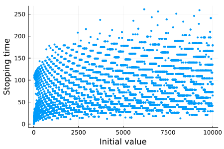
endJust for fun, let's plot the stopping time of the initial values from 1 to 10,000:
using Plots
plt = scatter(
    map(collatz_stopping_time, 1:10_000),
    xlabel = "Initial value",
    ylabel = "Stopping time",
    label = "",
    markercolor = 1,
    markerstrokecolor = 1,
    markersize = 3,
    size = (450, 300),
)
We can easily parallelize map(collatz_stopping_time, 1:10_000) and get a good speedup:
julia> Threads.nthreads()  # I started `julia` with `-t 4`
4

julia> using BenchmarkTools

julia> @btime map(collatz_stopping_time, 1:100_000);
  18.116 ms (2 allocations: 781.33 KiB)

julia> @btime Folds.map(collatz_stopping_time, 1:100_000);
  5.391 ms (1665 allocations: 7.09 MiB)
Iterator comprehensions
Julia's iterator comprehension syntax is a powerful tool for composing mapping, filtering, and flattening. Recall that mapping can be written as an array or iterator comprehension:
b1 = map(x -> x + 1, 1:3)
b2 = [x + 1 for x in 1:3]         # array comprehension
b3 = collect(x + 1 for x in 1:3)  # iterator comprehension
@assert b1 == b2 == b3
b1
3-element Vector{Int64}:
2
3
4The iterator comprehension can be executed with threads by using Folds.collect:
b4 = Folds.collect(x + 1 for x in 1:3)
@assert b1 == b4
🔬 Test Code
using Test
    @testset begin
        @test b1 == b2 == b3
    end
☑ Pass
Test Summary: | Pass  Total
test set      |    1      1
Note that more complex composition of mapping, filtering, and flattening can also be executed in parallel:
c1 = Folds.collect(y for x in 1:3 if isodd(x) for y in 1:x)4-element Vector{Int64}:
1
1
2
3Transducers.dcollect is for using iterator comprehensions with a distributed backend:
using Transducers
c2 = dcollect(y for x in 1:3 if isodd(x) for y in 1:x)
@assert c1 == c2
🔬 Test Code
@test c1 == c2 == [1, 1, 2, 3]☑ Pass
Pre-defined reductions
Functions such as sum, prod, maximum, and all are the examples of reduction (aka fold)[1] that can be parallelized. They are very powerful tools when combined with iterator comprehensions. Using Folds.jl, a sum of an iterator created by the comprehension syntax
d1 = sum(x + 1 for x in 1:3)9can easily be parallelized by
d2 = Folds.sum(x + 1 for x in 1:3)9🔬 Test Code
@test d1 == d2☑ Pass
For the full list of pre-defined reductions and other parallelized functions, type Folds. and press TAB in the REPL.
| [1] | map and collect are also fold.
|
Practical example: Maximum stopping time of Collatz function
We can use maximum to compute the maximum stopping time of Collatz function on a given the range of initial values
max_time = Folds.maximum(collatz_stopping_time, 1:100_000)350🔬 Test Code
@test max_time == 350☑ Pass
We get a speedup similar to the map example above:
julia> @btime maximum(collatz_stopping_time, 1:100_000)
  17.625 ms (0 allocations: 0 bytes)
350

julia> @btime Folds.maximum(collatz_stopping_time, 1:100_000)
  5.024 ms (1214 allocations: 69.17 KiB)
350
OnlineStats.jl
OnlineStats.jl provides a very rich and composable set of reductions. You can pass it as the first argument to Folds.reduce:
using OnlineStats: Mean
e1 = Folds.reduce(Mean(), 1:10)
Mean: n=10 | value=5.5🔬 Test Code
using Test, OnlineStats; @test e1 == fit!(Mean(), 1:10)☑ Pass
💡 Note
While OnlineStats.jl often does not provide the fastest way to compute the given statistics when all the intermediate data can fit in memory, in many cases you don't really need the absolute best performance. However, it may be worth considering other ways to compute statistics if Folds.jl + OnlineStats.jl becomes the bottleneck.
Manual reductions
For non-trivial parallel computations, you need to write a custom reduction. FLoops.jl provides a concise set of syntax for writing custom reductions. For example, this is how to compute sums of two quantities in one sweep:
using FLoops

@floop for (x, y) in zip(1:3, 1:2:6)
    a = x + y
    b = x - y
    @reduce(s += a, t += b)
end
(s, t)
(15, -3)🔬 Test Code
@test (s, t) == (15, -3)☑ Pass
In this example, we do not initialize s and t; but it is not a typo. In parallel sum, the only reasonable value of the initial state of the accumulators like s and t is zero. So, @reduce(s += a, t
+= b) works as if s and t are initialized to appropriate type of zero. However, since there are many zeros in Julia (0::Int, 0.0::Float64, (0x00 + 0x00im)::Complex{UInt8}, ...), s and t are undefined if the input collection (i.e., the value of xs in for
x in xs) is empty.
To control the type of the accumulators and also to avoid UndefVarError in the empty case, you can set the initial value with accumulator = initial_value op input syntax
@floop for (x, y) in zip(1:3, 1:2:6)
    a = x + y
    b = x - y
    @reduce(s2 = 0.0 + a, t2 = 0im + b)
end
(s2, t2)
(15.0, -3 + 0im)🔬 Test Code
@test (s2, t2) === (15.0, -3 + 0im)☑ Pass
To understand the computation of @floop with @reduce(accumulator =
initial_value op input) syntax, you can get a rough idea by just ignoring @reduce( and corresponding ,s and ). More concretely:
Extract expressions
accumulator = initial_value("initializers") fromaccumulator = initial_value op inputand put them in front of theforloop.Convert
accumulator = initial_value op inputto inplace updateaccumulator = accumulator op input.Strip off
@reduce.
So, the above example of @floop is equivalent to
let
    s2 = 0.0  # initializer
    t2 = 0im  # initializer
    for (x, y) in zip(1:3, 1:2:6)
        a = x + y
        b = x - y
        s2 = s2 + a  # converted from `s2 = 0.0 + a` in `@reduce`
        t2 = t2 + b  # converted from `t2 = 0im + b` in `@reduce`
    end      # \
    (s2, t2) #  `- the first arguments are now same as the left hand sides
end
(15.0, -3 + 0im)🔬 Test Code
@test (s3, t3) === (s2, t2)☑ Pass
The short-hand version @reduce(s += a, t += b) is implemented by using the first element of the input collection as the initial value.
This transformation is used for generating the base case that is executed in a single Task. Multiple results from tasks are combined by the operators and functions specified by @reduce. More explicitly, (s2_right, t2_right) is combined into (s2_left,
t2_left) by
s2_left = s2_left + s2_right
t2_left = t2_left + t2_right
⚠ Warning
Don't use locks or atomics! (unless you know what you are doing)
In particular, do not write
acc = Threads.Atomic{Int}(0)
Threads.@thread fors x in xs
    Threads.atomic_add!(acc, x + 1)
end
Locks and atomics help you write correct concurrent programs when used appropriately. However, they do so by limiting parallel execution. Using data parallel pattern is the easiest way to get high performance.
Parallel findmin/findmax with @reduce() do
@reduce() do syntax is the most flexible way in FLoops.jl for expressing custom reductions. It is very useful when one variable can influence other variable(s) in reduction (e.g., index and value in the example below). Note also that @reduce can be used multiple times in the loop body. Here is a way to compute findmin and findmax in parallel:
@floop for (i, x) in pairs([0, 1, 3, 2])
    @reduce() do (imin = -1; i), (xmin = Inf; x)
        if xmin > x
            xmin = x
            imin = i
        end
    end
    @reduce() do (imax = -1; i), (xmax = -Inf; x)
        if xmax < x
            xmax = x
            imax = i
        end
    end
end

@show imin xmin imax xmax
imin = 1
xmin = 0
imax = 3
xmax = 3
🔬 Test Code
@test (imin, xmin, imax, xmax) == (1, 0, 3, 3)☑ Pass
We can understand the computation of @floop roughly by ignoring the lines with @reduce() do and corresponding end. More concretely:
Extract expressions
accumulator = initial_value("initializers") from(accumulator = initial_value; input)or(accumulator; input)and put them in front of theforloop.Remove
@reduce() do ...and correspondingend.
let
    imin2 = -1    # -+
    xmin2 = Inf   #  | initializers
    imax2 = -1    #  |
    xmax2 = -Inf  # -+

    for (i, x) in pairs([0, 1, 3, 2])
        if xmin2 > x   # -+
            xmin2 = x  #  | do block bodies
            imin2 = i  #  |
        end            #  |
        if xmax2 < x   #  |
            xmax2 = x  #  |
            imax2 = i  #  |
        end            # -+
    end

    @show imin2 xmin2 imax2 xmax2
end
imin2 = 1
xmin2 = 0
imax2 = 3
xmax2 = 3
🔬 Test Code
@test (imin2, xmin2, imax2, xmax2) == (1, 0, 3, 3)☑ Pass
The above computation is used for each partition of the input collection and combined by the reducing function defined by @reduce()
do block. That is to say, (imin2_right, xmin2_right, imax2_right,
xmax2_right) is combined into (imin2_left, xmin2_left, imax2_left,
xmax2_left) by
if xmin_left > xmin_right
xmin_left = xmin_right
imin_left = imin_right
end
if xmax_left < xmax_right
xmax_left = xmax_right
imax_left = imax_right
endRemark: Observe that x and i of the first @reduce() do block are replaced with xmin_right and imin_right while x and i of the second @reduce() do block are replaced with xmax_right and imax_right. This is why we used two @reduce() do blocks; we need to "pair" x/i with xmin/imin or with xmax/imax depending on which if block we are in.
Parallel findmin/findmax with Folds.reduce (tedious!)
Note that it is not necessary to use @floop for writing a custom reduction. For example, you can write an equivalent code with Folds.reduce:
(imin3, xmin3, imax3, xmax3) = Folds.reduce(
((i, x, i, x) for (i, x) in pairs([0, 1, 3, 2]));
init = (-1, Inf, -1, -Inf)
) do (imin, xmin, imax, xmax), (i1, x1, i2, x2)
if xmin > x1
xmin = x1
imin = i1
end
if xmax < x2
xmax = x2
imax = i2
end
return (imin, xmin, imax, xmax)
end
@assert (imin3, xmin3, imax3, xmax3) == (imin, xmin, imax, xmax)
🔬 Test Code
@test (imin3, xmin3, imax3, xmax3) == (imin, xmin, imax, xmax)☑ Pass
However, as you can see, it is much more verbose and error-prone (e.g., the initial values and the variables are declared in different place).
Histogram with reduce
mapreduce and reduce are useful when combining pre-existing operations. For example, we can easily implement histogram by combining mapreduce, Dict, and mergewith!:
str = "dbkgbjkahbidcbcfhfdeedhkggdigfecefjiakccjhghjcgefd"
f1 = mapreduce(x -> Dict(x => 1), mergewith!(+), str)Dict{Char, Int64} with 11 entries:
'f' => 5
'd' => 6
'e' => 5
'j' => 4
'h' => 5
'i' => 3
'k' => 4
'a' => 2
'c' => 6
'g' => 6
'b' => 4Note that this code has a performance problem: Dict(x => 1) allocates an object for each iteration. This is bad in particular in threaded Julia code because it frequently invokes garbage collection. To avoid this situation, we can replace Dict with MicroCollections.SingletonDict which does not allocate the dictionary in the heap. SingletonDict can be "upgraded" to a Dict by calling BangBang.mergewith!!. It will then create a mutable object for each task to mutate. We can then compose an efficient parallel histogram operation:
using BangBang: mergewith!!
using MicroCollections: SingletonDict
f2 = Folds.mapreduce(x -> SingletonDict(x => 1), mergewith!!(+), str)
@assert f1 == f2
🔬 Test Code
@test f1 == f2☑ Pass
(For more information, see Transducers.jl's ad-hoc histogram tutorial.)
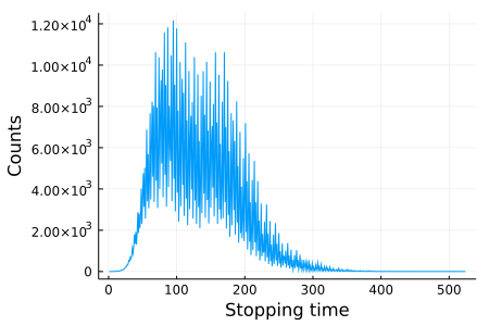
Practical example: Histogram of stopping time of Collatz function
Let's compute the histogram of collatz_stopping_time over some range of initial values. Unlike the histogram example above, we know that the stopping time is a positive integer. So, it makes sense to use an array as the data structure that maps a bin (index) to a count. There is no pre-defined reducing function like mergewith! we can use. Fortunately, it is easy to write it using @reduce() do syntax in @floop:
using FLoops
using MicroCollections: SingletonDict
maxkey(xs::AbstractVector) = lastindex(xs)
maxkey(xs::SingletonDict) = first(keys(xs))
function collatz_histogram(xs, executor = ThreadedEx())
@floop executor for x in xs
n = collatz_stopping_time(x)
n > 0 || continue
obs = SingletonDict(n => 1)
@reduce() do (hist = Int[]; obs)
l = length(hist)
m = maxkey(obs) # obs is a Vector or SingletonDict
if l < m
# Stretch `hist` so that the merged result fits in it.
resize!(hist, m)
fill!(view(hist, l+1:m), 0)
end
# Merge `obs` into `hist`:
for (k, v) in pairs(obs)
@inbounds hist[k] += v
end
end
end
return hist
endAs we discussed above, @reduce() do blocks are used in two contexts; for the sequential base case and for combining the accumulated results from two base cases. Thus, for combining hist_left and hist_right, we need to substitute hist_right to obs. This is why we need to handle the cases where obs is a SingletonDict and a Vector. Thanks to multiple dispatch, it is very easy to absorb the difference in the two containers. We can just use what Base defines for pairs and only need to define maxkey for absorbing the remaining difference.
💡 Note
When writing
@reduce() do (L₁ = I₁; R₁), (L₂ = I₂; R₂), ..., (Lₙ =
Iₙ; Rₙ)
, make sure that the do block body can handle arbitrary possible value of Lᵢ substituted to Rᵢ and not just Rᵢs that are calculated directly in the for loop body.Example usage:
using Plots
plt = plot(
    collatz_histogram(1:1_000_000),
    xlabel = "Stopping time",
    ylabel = "Counts",
    label = "",
    size = (450, 300),
)
We use @floop executor for ... syntax so that it is easy to switch between different kind of execution mechanisms; i.e., sequential, threaded, and distributed execution:
hist1 = collatz_histogram(1:1_000_000, SequentialEx())
hist2 = collatz_histogram(1:1_000_000, ThreadedEx())
hist3 = collatz_histogram(1:1_000_000, DistributedEx())
@assert hist1 == hist2 == hist3
🔬 Test Code
@test hist1 == hist2 == hist3☑ Pass
For example, we can easily compare the performance of sequential and threaded execution:
julia> @btime collatz_histogram(1:1_000_000, SequentialEx());
  220.022 ms (9 allocations: 13.81 KiB)

julia> @btime collatz_histogram(1:1_000_000, ThreadedEx());
  58.271 ms (155 allocations: 60.81 KiB)
Quick notes on @threads and @distributed
Julia itself has Threads.@threads macro for threaded for loop and @distributed macro for distributed for loop. They are adequate for simple use cases but come with some limitations. For example, @threads does not have built-in reducing function support. Although @distributed macro has reducing function support, it is limited to pre-defined functions and it is tedious to handle multiple variables. Both of these macros only have simple static scheduler and lacks an option like basesize supported by FLoops.jl and Folds.jl to tune load balancing. Furthermore, the code written with @threads cannot be reused for @distributed and vice versa.
Next steps
Hopefully, this tutorial covers a bare minimum for you to start writing data-parallel programs and the documentations of FLoops.jl and Folds.jl are now a bit more accessible. These two libraries are based on the protocol designed for Transducers.jl which also contains various tools for data parallelism.
Transducers.jl's parallel processing tutorial covers a similar topic with explanations for more low-level details. Parallel word count tutorial based on Guy L. Steele Jr.'s 2009 ICFP talk is more advanced but I find it a very good example to follow for understanding what is possible with a clever design of the reducing function.
Note that ideas presented in this tutorial are very general and should be applicable also when using other libraries. For example, the idea of custom reduction is useful in GPU computing when using mapreduce on CuArray.
See also:

© Takafumi Arakaki. Last modified: June 10, 2021. Website built with Franklin.jl and the Julia programming language.